Implementing K Nearest Neighbors on CIFAR-10
9/7/21
Introduction
The purpose of this was to familiarize myself further with PyTorch and in general, tensor operations. Credit to UMichigan's 498/598 Deep Learning for Computer Vision - I use some of their code.
CIFAR-10 is a well known dataset composed of 60,000 colored 32x32 images. kNN classification is an algorithm to classify inputs by comparing their similarities to a training set accompanied with labels. There is the very similar kNN Regression, which employs the same idea, just different task. The next section "What is kNN / How does kNN work" assumes the reader has no prior understanding of kNN. The sections following, "Loading CIFAR" and beyond, assumes the reader to have basic understanding of Python, PyTorch, and Linear Algebra. If you aren't familiar with these concepts but have read the "What is kNN / How does kNN work" section, then you may still be good. I will toss in some explanations in blue for important things.
What is kNN / How does kNN work
I broadly defined kNN above. This section is going to be dedicated to explaining further what kNN classification does, and how it works. I'm going to be using images as an example dataset to aid my explanation of kNN. Throughout this read, I frequently use "test", "unlabeled", and "input" interchangeably to refer to the input for kNN. Feel free to skip this section if you're just interested in the code and implementation. Feel free to also only read this section if you just want a synopsis of kNN classification.
The goal is classification. We have a dataset, images in our case, and unfortunately a portion of the images are unlabeled - they do not have an accompanying label which classifies them. kNN is a method to "intelligibly" label the unclassified images by computing similarity with the labeled images. Euclidean distance is a popular metric to quantify the similarities, however there are a handful of other measures that have their own idiosyncrasies (Manhattan & Minkowsi). In the case of images, kNN computes the Euclidean distance between an unlabled and labeled image by iterating over their pixel values. The unlabeled image then takes the same majority classification as its k nearest neighbors or k neighbors with the lowest Euclidean distance, where k is a hyperparameter. This process produces a loop where each unlabeled input image is compared to every labeled image in the dataset by their pixel values. Once the first unlabeled image iterates through the entire labeled training set, the algorithm then moves onto the next image in the test set to do it all again.
Visualization of computing the pixel values of a single test image (left) against every train image (right).
Right click and toggle 'show controls' to stop the animation.
For reference, the Euclidean distance is: √∑ni=1(xi−yi)2. In the visualization above, kNN is operating on a colored (RGB) image dataset of 5x5 pixels - so in total 75 pixels per image (3x5x5). To compute the Eucliden distance between one test image and one training image, the squared difference between corresponding pixels in both images are taken and then then summed and finally taken the square root of. To reiterate, we are taking 75 differences, squaring each one, summing all that together, and then finally square rooting everything. And this occurs for each test image against every training image. It's worth mentioning, in the animation I do not show the 5x5 green and blue pixel channels being iterated over like I did for the red channel; instead the green and blue layers are simplified with a single "blink".
As mentioned briefly before, the k in kNN is an integer hyperparameter that says how many neighbors our test image should pay attention to. It tells each test image to find their k nearest neighbors of a particular label, then label them in accordance with those neighbors. If k = 1, then we're asking kNN to classify every test image with it's closest single neighbor. If k = 3, then we're asking kNN to classify a test image with it's 3 closest neighbors (lowest Euclidean distance) of the same class. Some considerations when picking a value for k is to not pick a value that would result in a tie - where the k closest neighbors are an even distribution between different classes. This can generally be avoided by 1) picking odd numbers for k and 2) not picking multiples of the number of classes. Below is a visualization for different values of k. Hyperparameter definition.
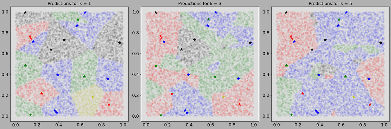
The stars reference labeled images and the translucent dots reference unlabled images.
Setting Up
Loading CIFAR-10
Lets now look at using kNN on CIFAR-10. Our data is going to be stored simply in the four variables: x_train, x_test, y_train, and y_test. They are declared simply with:
   x_train, y_train, x_test, y_test = cifar10()
   """
   x_train: shape (B, C, H, W) tensor where B is batch size, C is channel size, H
      is height, and W is width.
   y_train: shape (B) tensor where B is batch size.
   x_test: shape (B, C, H, W) tensor where B is batch size, C is channel size, H
      is height, and W is width.
   y_test: shape(B) tensor where B is batch size.
   """


   # Training Set.
   # x_train is composed of 50,000 images where y_train references the corresponding labels
   print('data shape:', x_train.shape)
   print('labels shape:', y_train.shape)
   # >>> data shape: torch.Size([50000, 3, 32, 32])
   # >>> labels shape: torch.Size([50000])

   # Test Set
   # x_test is composed of 10,000 images where y_test references the corresponding labels
   print('data shape:', x_test.shape)
   print('labels shape', y_test.shape)
   # >>> data shape: torch.Size([10000, 3, 32, 32])
   # >>> labels shape: torch.Size([10000])
Below is the cifar10() definition. It isn't necessary to understand kNN's but I thought it was worth adding for the curious. You can see it above in the comments: x_train returns a 4 dimensional tensor composed of 50,000 3x32x32 training images, y_train returns a 1 dimensional tensor composed of corresponding labels for those 50,000 images, x_test returns a 10,000 3x32x32 testing images, and lastly y_test returns the corresponding labels for those 10,000 images. I refer to the training dataset as "unlabeled" despite having a tensor, y_train, of labels because we will only use those labels to determine the final accuracy of our kNN algorithm.
   import os
   import torch
   from torchvision.datasets import CIFAR10

   def _extract_tensors(dset, num=None):
      x = torch.tensor(dset.data, dtype=torch.float32).permute(0, 3, 1, 2).div_(255)
      y = torch.tensor(dset.targets, dtype=torch.int64)
      if num is not None:
         if num <= 0 or num > x.shape[0]:
            raise ValueError('Invalid value num=%d; must be in the range [0, %d]'
                           % (num, x.shape[0]))
         x = x[:num].clone()
         y = y[:num].clone()
      return x, y

   def cifar10(num_train=None, num_test=None):
      download = not os.path.isdir('cifar-10-batches-py')
      dset_train = CIFAR10(root='.', download=download, train=True)
      dset_test = CIFAR10(root='.', train=False)
      x_train, y_train = _extract_tensors(dset_train, num_train)
      x_test, y_test = _extract_tensors(dset_test, num_test)

      return x_train, y_train, x_test, y_test
Visualizing CIFAR-10
To see what we're working with, here are a 12 random images from each class with their corresponding label to the left:

Each image is composed of 3x32x32 pixel values. The 3x32x32 references their height/width and the 3x32x32 references the color channels, which most of computer vision (to my knowledge) use RGB. The labels are simply a tensor of integers ranging from [0,9]. Each integer serves as an index to a corresponding list of classes:
   classes = ['plane', 'car', 'bird', 'cat', 'deer', 'dog', 'frog', 'horse', 'ship', 'truck']
   # plane = 0, car = 1, bird = 2 ... truck = 9

   print(x_train[0].shape)
   # >>> torch.Size([3, 32, 32])

   # Finding integer label of corresponding 0th image
   print(y_train[0])
   # >>> tensor(6)
   # Element 6 in 'classes' list is a frog (which is correct, just take my word for it)
Subsampling
Before actually implementing kNN, iterating over 60000 images and labels when testing code is exhaustive. To keep my 1070 GPU happy, I subsampled. Subsampling takes a small portion of the whole dataset to work with while building the kNN. Doing this, I no longer had my computer run through the entire dataset each time I tested code. We subsample using the parameters provided in cifar10(). We can set these to any integer value to determine the size of the subsample. These will be the tensors we work with while building the kNN algorithm.
   # Subsample size
   num_train = 500
   num_test = 250

   # Redeclaring x_train...y_test with subsample
   x_train, y_train, x_test, y_test = cifar10(num_train, num_test)

   print('data shape:', x_train.shape)
   print('labels shape:', y_train.shape)
   # Training set:
   # >>> data shape: torch.Size([500, 3, 32, 32])
   # >>> labels shape: torch.Size([500])

   print('data shape:', x_test.shape)
   print('labels shape:', y_test.shape)
   # Testing set:
   # >>> data shape: torch.Size([250, 3, 32, 32])
   # >>> labels shape: torch.Size([250])
Building kNN
Finding the Euclidean distance
Everything is set - we've preprocessed and subsampled our dataset. I'm going to show a couple ways to find the Euclidean distance between testing and training images. The first is with using nested loops to populate our output matrix dists, where each loop will iterate over an axis. Although this method is not very efficient because it does not make use of broadcasting, I think it's helpful from a pedagogical standpoint. A more efficient representation, compute_distances_no_loops is shown immediately below. It is worth mentioning that PyTorch does have functions designed to do this already such as: torch.cdist, but I'm also going to refrain from using them. Broadcasting is a term that enables arithmetic for tensors of different dimensionality, read more here.
   def compute_distances_two_loops(x_train, x_test):
      """
      Inputs:
      x_train: shape (num_train, C, H, W) tensor.
      x_test: shape (num_test, C, H, W) tensor.

      Returns:
      dists: shape (num_train, num_test) tensor where dists[j, i] is the
         Euclidean distance between the ith training image and the jth test
         image.
      """

      # Get the number of training and testing images
      num_train = x_train.shape[0] # (500)
      num_test = x_test.shape[0] # (250)


      # dists will be the tensor housing all distance measurements between testing and training
      dists = x_train.new_zeros(num_train, num_test) # (500, 250)

      # Flatten tensors
      train = x_train.flatten(1) # (500, 3072)
      test = x_test.flatten(1) # (250, 3072)

      # Find Euclidean distance using loops
      for i in range(num_test):
         for j in range(num_train):
            dists[j, i] = torch.sqrt(torch.sum(torch.square(train[j] - test[i])))


      return dists
As stated before, CIFAR-10 images are 3x32x32. The entire training dataset can be represented with a tensor of shape [50000, 3, 32, 32]. Because of our subsampling, we drastically reduce the training size to [500, 3, 32, 32]. We flatten both the the x_train and x_test tensors to transform our [500, 3, 32, 32] and [250, 3, 32, 32] training image tensor into [500, 3072] and [250, 3072] tensors respectively. Now you can think of our reshaped tensors as matrices where each row houses every single pixel value (3x32x32) of an image. The purpose of flattening can be thought of as the final preprocessing step before we compute the Euclidean distance using two loops.
The first for loop iterates over every test image. The second iterates over every training image. Like discussed before, it computes the Euclidean distance between the jth training image and ith testing image two and populates the dists tensor in its respective position.
Here is a more efficient variation of finding the Euclidean distance that has no loops and instead makes use of broadcasting:
   def compute_distances_no_loops(x_train, x_test):
      """
      Inputs:
      x_train: shape (num_train, C, H, W) tensor.
      x_test: shape (num_test, C, H, W) tensor.

      Returns:
      dists: shape (num_train, num_test) tensor where dists[i, j] is the
         Euclidean distance between the ith training image and the jth test
         image.
      """
      # Get number of training and testing images
      num_train = x_train.shape[0]
      num_test = x_test.shape[0]

      # Create return tensor with desired dimensions
      dists = x_train.new_zeros(num_train, num_test) # (500, 250)

      # Flattening tensors
      train = x_train.flatten(1) # (500, 3072)
      test = x_test.flatten(1) # (250, 3072)

      # Find Euclidean distance
      # Squaring elements
      train_sq = torch.square(train)
      test_sq = torch.square(test)

      # Summing row elements
      train_sum_sq = torch.sum(train_sq, 1) # (500)
      test_sum_sq = torch.sum(test_sq, 1) # (250)

      # Matrix multiplying train tensor with the transpose of test tensor
      mul = torch.matmul(train, test.transpose(0, 1)) # (500, 250)

      # Reshape enables proper broadcasting.
      # train_sum_sq = [500, 1] shape tensor and test_sum_sq = [1, 250] shape tensor.
      # This enables broadcasting to match desired dimensions of dists
      dists = torch.sqrt(train_sum_sq.reshape(-1, 1) + test_sum_sq.reshape(1, -1) - 2*mul)

      return dists
This procedure makes use of expanding the square in the Euclidean distance:
On this no-loop variant of computing the Euclidean, we are evaluating all arithmetic independently and then compiling everything together so that it represents the right hand side of the formula above. Instead of going through element by element, after we preprocess the inputs, we square the train and test tensors immediately then take the sum of their rows. Then, $x_iy_i$ is evaluated through the matrix multiplication of the train [500, 3072] and the transpose of the test [3072, 250] tensors. Finally, we have all terms to produce the right hand of the equality above, allowing us to wrap everything in a square root and store it in dists. Within each column of dists is the Euclidean distance of every training image with respect to a test image. For comparison, the two loop version takes (for me) 7.27 seconds. The no loop version takes 0.02 seconds. The no loop version is 455.7x faster than the two loop. This probably provides better intuition behind how powerful broadcasting (and matmul) can be.
Classifying our test images
Using the compute_distances_no_loops function, we can now build a classifier. I will be focusing on the predict method. check_accuracy is simply to determine how well our classifier performs.
   class KnnClassifier:
      def __init__(self, x_train, y_train):
         """
         x_train: shape (num_train, C, H, W) tensor where num_train is batch size,
            C is channel size, H is height, and W is width.
         y_train: shape (num_train) tensor where num_train is batch size providing labels
         """

         self.x_train = x_train
         self.y_train = y_train

      def predict(self, x_test, k=1):
         """
         x_test: shape (num_test, C, H, W) tensor where num_test is batch size,
            C is channel size, H is height, and W is width.
         k: The number of neighbors to use for prediction
         """

         # Init output shape
         y_test_pred = torch.zeros(x_test.shape[0], dtype=torch.int64)

         # Find & store Euclidean distance between test & train
         dists = compute_distances_no_loops(self.x_train, x_test)

         # Index over test images
         for i in range(dists.shape[1]):
            # Find index of k lowest values
            x = torch.topk(dists[:,i], k, largest=False).indices

            # Index the labels according to x
            k_lowest_labels = self.y_train[x]

            # y_test_pred[i] = the most frequent occuring index
            y_test_pred[i] = torch.argmax(torch.bincount(k_lowest_labels))

         return y_test_pred

      def check_accuracy(self, x_test, y_test, k=1, quiet=False):
         """
         x_test: shape (num_test, C, H, W) tensor where num_test is batch size,
            C is channel size, H is height, and W is width.
         y_test: shape (num_test) tensor where num_test is batch size providing labels
         k: The number of neighbors to use for prediction
         quiet: If True, don't print a message.

         Returns:
         accuracy: Accuracy of this classifier on the test data, as a percent.
            Python float in the range [0, 100]
         """

         y_test_pred = self.predict(x_test, k=k)
         num_samples = x_test.shape[0]
         num_correct = (y_test == y_test_pred).sum().item()
         accuracy = 100.0 * num_correct / num_samples
         msg = (f'Got {num_correct} / {num_samples} correct; '
               f'accuracy is {accuracy:.2f}%')
         if not quiet:
            print(msg)
         return accuracy
The goal is to return a tensor y_test_pred where the ith index is the assigned label to ith test image by the kNN algorithm. Below is a visualization of how the classification works on a dists of size [5x3]. The algorithm finds the index of the k lowest Euclidean distances within each column. Then it corresponds that index with self.y_train and stores those values in k_lowest_labels. y_test_pred[i] is then assigned the most frequent occuring label present in k_lowest_labels. Once a column calculates it's value for y_test_pred, it proceeds to the next. Each column can be thought of as a test image and every element in the column represents the Euclidean distance between that test image with every training image.
Right click and toggle 'show controls' to stop the animation.
We've finished implementing kNN and can begin testing the algorithm on larger portions of the dataset to see how well it performs. With k set to 5, 5000 training images, and 500 testing images, our kNN results in a 27.8% accuracy for proper classification on a portion of the CIFAR-10 dataset. It's certainly no convolutional neural network, however it shows how far computer vision has come (kNN was developed in 1951).
   from knn import KnnClassifier

   torch.manual_seed(0)
   num_train = 5000
   num_test = 500
   x_train, y_train, x_test, y_test = cifar10(num_train, num_test)

   classifier = KnnClassifier(x_train, y_train)
   classifier.check_accuracy(x_test, y_test, k=5)
   # >>> Got 139 / 500 correct; accuracy is 27.80%
   # >>> 27.8
Cross Validation
A problem with the current kNN is that after we've successfully automated a process of "intelligebly" classifying images, we are still left with "guessing" the best k for the algorithm. As our algorithm currently exists, we have to manually tune the hyperparameter k to some integer value, which raises the question - is that the best value for k? Cross validation is a procedure to automate selecting an optimal value for k. The problem with this is that to evaluate the efficacy of some value k, we currently use the test set. If we want to evaluate numerous values for k it breaks the convention of segregating the test set until final testing. Finding some optimal k through using the same test set on each evaluation, would have our kNN algorithm fall victim to overfitting. Our model would be too well trained to the test set, and because of this, may not generalize well to new and unseen data. Overfitting is a big issue in training. The inverse of overfitting is underfitting, where a model does not yield high enough or desired efficacy on training data.
Cross validation further segregates our training set into "chunks". For our subsample of 5,000 test images and labels, we can create 5 tensors of shape [1,000, 3072]. One of those 5 chunks becomes what is called the validation set to evaluate an optimal k. The validation set does the job of the previously defined test set. By partioning our data, we circumvent the issue of overfitting - our test set is untouched until the final...test.
   def knn_cross_validate(x_train, y_train, num_folds=5, k_choices=None):
      """
      Inputs:
      x_train: Tensor of shape (num_train, C, H, W) giving all training data
      y_train: int64 tensor of shape (num_train,) giving labels for training data
      num_folds: Integer giving the number of folds to use
      k_choices: List of integers giving the values of k to try

      Returns:
      k_to_accuracies: Dictionary mapping values of k to lists, where
         k_to_accuracies[k][i] is the accuracy on the ith fold of a KnnClassifier
         that uses k nearest neighbors.
      """
      # Create a list of k's for testing
      if k_choices is None:
         k_choices = [1, 3, 5, 8, 10, 12, 15, 20, 50, 100]

      # Create empty lists to house the chunks for cross validation
      x_train_folds = []
      y_train_folds = []

      # Flatten x_train from [5000, 3, 32, 32] to [5000, 3072]
      x_train_flat = x_train.view(x_train.shape[0], -1)

      # Partition our training set to 5 tensors of training images of shape [1000, 3072] and 5 labels of shape [1000]
      x_train_folds = torch.chunk(x_train_flat, num_folds, dim=0)
      y_train_folds = torch.chunk(y_train, num_folds, dim=0)

      # Create object to house the combination of accuracies for different values k for different validation sets
      k_to_accuracies = {}

      # Iterate through every combination of k_choices and possible validation sets
      for k in k_choices:
         for folds in range(num_folds):
            # Setting validation sets
            x_valid = x_train_folds[folds]
            y_valid = y_train_folds[folds]

            # Setting new training sets
            x_traink = torch.cat(x_train_folds[:folds] + x_train_folds[folds + 1:])
            y_traink = torch.cat(y_train_folds[:folds] + y_train_folds[folds + 1:])

            # Call our kNN with the newly defined sets
            knn = KnnClassifier(x_traink, y_traink)

            # Check accuracy
            accuracy = knn.check_accuracy(x_valid, y_valid, k=k)

            # Append a list of accuracies for different values k to k_to_accuracies
            k_to_accuracies.setdefault(k, []).append(accuracy)

            return k_to_accuracies

   # Accuracies when running cross validation on our subsample
   # >>> k = 1 got accuracies: [26.3, 25.7, 26.4, 27.8, 26.6]
   # >>> k = 3 got accuracies: [23.9, 24.9, 24.0, 26.6, 25.4]
   # >>> k = 5 got accuracies: [24.8, 26.6, 28.0, 29.2, 28.0]
   # >>> k = 8 got accuracies: [26.2, 28.2, 27.3, 29.0, 27.3]
   # >>> k = 10 got accuracies: [26.5, 29.6, 27.6, 28.4, 28.0]
   # >>> k = 12 got accuracies: [26.0, 29.5, 27.9, 28.3, 28.0]
   # >>> k = 15 got accuracies: [25.2, 28.9, 27.8, 28.2, 27.4]
   # >>> k = 20 got accuracies: [27.0, 27.9, 27.9, 28.2, 28.5]
   # >>> k = 50 got accuracies: [27.1, 28.8, 27.8, 26.9, 26.6]
   # >>> k = 100 got accuracies: [25.6, 27.0, 26.3, 25.6, 26.3]

A total of 50 different accuracies result from our 10 different k's and 5 partitions from cross validation. We'd now like kNN to select the value for k that yielded the highest average accuracy for the 5 folds. We can see on the graph above, a k of around 12 provides the highest average. Below returns the k that has the highest average.
   def knn_get_best_k(k_to_accuracies):
      """
      Inputs:
      - k_to_accuracies: Dictionary mapping values of k to lists, where
      k_to_accuracies[k][i] is the accuracy on the ith fold of a KnnClassifier
      that uses k nearest neighbors.

      Returns:
      - best_k: best (and smallest if there is a conflict) k value based on
      the k_to_accuracies info
      """
      # Create best_k variable to return optimal k
      best_k = 0

      # Get keys and values from k_to_accuracies object
      keys = [k for k in k_to_accuracies.keys()]
      # >>> keys = [1, 3, 5, 8, 10, 12, 15, 20, 50, 100]
      values = [v for v in k_to_accuracies.values()]
      # >>> values = [[26.3, 25.7, 26.4, 27.8, 26.6], ..., [25.6, 27.0, 26.3, 25.6, 26.3]]

      # Get largest average of all the values
      max_avg = torch.argmax(torch.mean(torch.tensor(values), dim=1))
      # Get corresponding k for max_avg
      best_k = keys[max_avg]

      return best_k

      # >>> Best k is  10
      # >>> Got 141 / 500 correct; accuracy is 28.20%
      # >>> 28.2
Running on the entire CIFAR-10
We've finished creating our kNN algorithm which also makes use of cross validation to pick an optimal k based off the validation sets. Now we can finally operate on the entire CIFAR-10 dataset. If you have clicked to here from a Google search and are quickly looking to find the relevant code for kNN, it's in Classifying our test images.
   from knn import KnnClassifier

   torch.manual_seed(0)
   x_train_all, y_train_all, x_test_all, y_test_all = cifar10()

   classifier = KnnClassifier(x_train_all, y_train_all)
   classifier.check_accuracy(x_test_all, y_test_all, k=best_k)

   # >>> Got 3399 / 10000 correct; accuracy is 33.99%
   # >>> 33.99
Thoughts
Writing this took a bit longer than I expected. I tried to be intentionally redundant at times to solidify understanding of concepts that, when I learned kNN and some ML in general, had trouble understanding. I mentioned this at the top, but a large credit of my writing this goes to UMichigan's 498/598 Deep Learning for Computer Vision. If you're interested in making a kNN yourself, you can find the files there or analogously, you can find a NumPy variation through Stanford's CS231n. If you notice any typos, inconsistencies, or have thoughts in general, feel free to ping me and let me know.
- Ryan Lin