A Thorough Explanation to Recurrent Neural Networks

Introduction

Just as how a CNN's specialty is processing grid-like data such as images, a RNN specializes in procesing sequential data - data that is discretized. A very common example of a sequence could be a sentence. Each word in a sentence stands wholly on its own but when strung together constitute something new. Depending on the design and intended use of the RNN, we can parse a sequence in a handful of different ways. This "parsing" is specifically sequence processing, which I briefly talk about soon. I want to mention this now however since there is a lot of nuance in the math between different types of sequence processing. Because of this, the sections Forward Pass Transformations and beyond presume the type of sequence shown immediately below called a many to many.

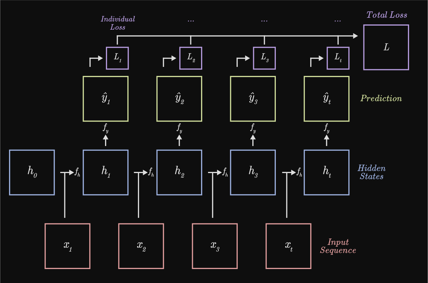
xt represents the input sequence, $h_t$ the hidden states, $y_t$ the prediction, and $L_t$, the individual loss.

A couple of "top level" things to look at. I discuss some of these points further below, but they're nice to acknowledge in the beginning - confusion is okay. One: every timestep function $f_h$ requires, as arguments, it's corresponding input $x_t$ and prior hidden state $h_{t - 1}$ to produce the next hidden state $h_t$. Two: The gradients in backpropagation will be summed at each step as RNNs use shared weights at every timestep. Three: both the input and output sequence, shown as red and yellow respectively, are arbitrarily partitioned t times. This is one of a "handful of different ways" to represent the input and output for an RNN. Four: a inital hidden state, $h_0$, must be provided for the forward pass of an RNN. The initial hidden state is either learnt (the output of network x can be used to to populate $h_0$ in RNN y ) or set to 0. Five: the total loss is a sum over every individual loss.

Sequence Processing

The picture above is referred to as a "many to many" RNN. Depending on the task of the network, there are different ways of processing the data. For the many to many shown above, consider a video as input where the frames of the video compose the sequence. $x_1$ would be the first frame, $x_2$ would be the second... and so on. For this type of many-to-many, our output at each timestep could then be some decision/classification based off the input at that same timestep. So our RNN would be producing some output for every frame of video. Below are different types of models for processing different sequences. Note that although labeling and some intricacies are omitted, the many to many show below is not the same as the one shown above.

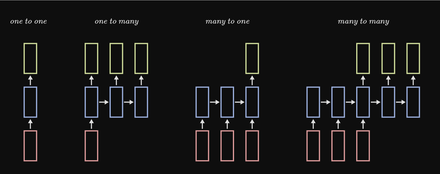
Examples: one to one: Image classification, one to many: Image captioning, many to one: Video classification, many to many: Machine translation
Captioning refers to a sequence of symbols. For image captioning our output would be a sequence of, ideally coherent, words describing what's happening in the image. Another example of a caption could be a sequence of letters, which at the end, would produce a word.

Forward Pass Transformations

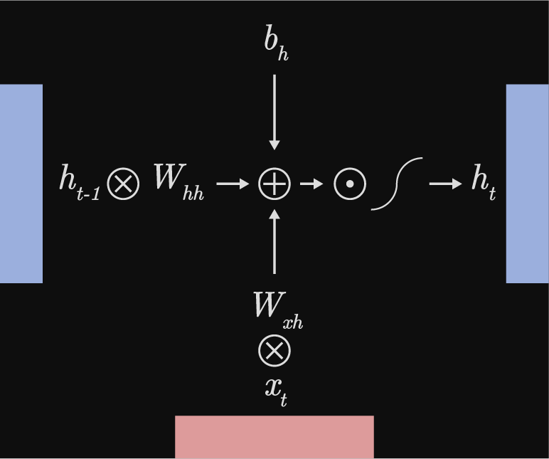
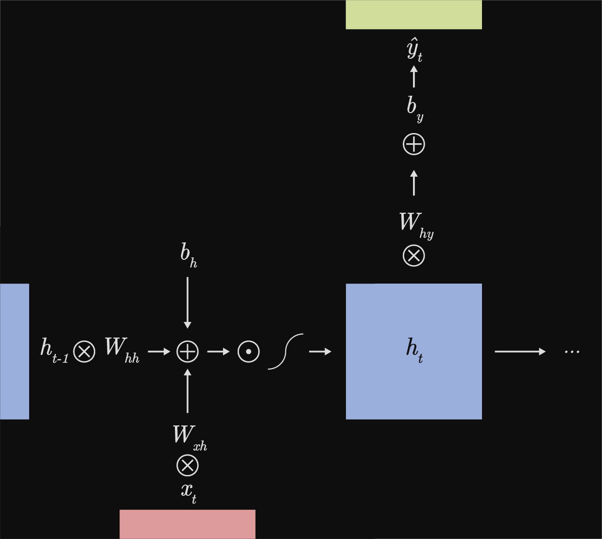
As mentioned above, a characteristic to RNNs is that weights are shared temporally, between all time steps. A simple Vanilla RNN can have three weight tensors: $W_{hh}$, $W_{xh}$, $W_{hy}$ and only a couple of bias parameters $b_h$ and $b_y$. Each of these parameters are recycled at each hidden step to compute either a local prediction or the next hidden step. It helps me to think of the index of tensors as $W_{(from)\;(to)}$ to visualize where that particular tensor belongs. Excluding the loss function, the two transformations shown below are fundamental to a Vanilla RNN.

Between hidden steps

Transformation between hidden steps $h_{t-1} \rightarrow h_t$: $$f_h(h_{t-1}, x_t) = h_t = tanh(W_{hh}h_{t-1} + W_{xh}x_t + b_h)$$

999

1

2

3

4

5

  def rnn_step_forward(x, prev_h, Wx, Wh, b):
      # Vanilla RNN uses tanh
      # torch.tanh(x) applies an element-wise activation over it's input
      next_h = torch.tanh(prev_h.mm(Wh) + x.mm(Wx) + b)
      return next_h

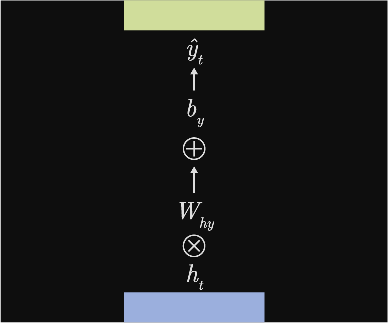
Between hidden steps & prediction

Transformation between hidden steps & prediction $h_{t} \rightarrow \hat{y}$: $$f_y(h_{t}) = \hat{y} = W_{hy}h_t + b_y$$

999

1

2

3

4

5

  def yhat(in_features, out_features, device, dtype):
      # Very simple linear transformation
      # https://pytorch.org/docs/stable/generated/torch.nn.Linear.html
      yhat = nn.Linear(in_features, out_features, device=device, dtype=dtype)
      return yhat

One Step Backwards

Combined picture of both computational graphs.

Time to go backwards. Before talking about anything, there are a handful of idiosyncrasies between the different sequence styles of RNNs. Everything below assumes a many to many sequence, very similar to the first picture at the top of this page. This is important because the process of computing some gradients is different between sequence styles.

I first show the process of only going back only a single hidden step. Afterwards I discuss fully propagating backwards t times to the first values.

Here are the partials we're looking for:

Here are the transformations again:

Above are the local gradients. The upstream gradient will be the derivative of the loss wrt to the prediction of the model at the subsequent timestep and will be represented as output_grad. We can now begin finding the desired gradients. Note that when differentiating wrt to a bias parameter, I sum along the Nth dimension to match the shape of said bias parameter.

Everything beyond $h_t$ runs through the element-wise tanh non-linearity so I create an intermediary variable which I will call $dtanh$ that uses a hyperbolic identity: $\frac{\mathrm{d}tanh(x)}{\mathrm{d}} = sech^2(x) = 1-tanh^2(x)$ to simplify finding the derivative since $tanh(x)$ is already provided to us in from the forward pass. For clarification, the x argument inside the tanh function is the argument in the forward pass at the current timestep.

  def oneStepBackwards(output_grad, cache):
      """
      Backward pass for a single timestep of a vanilla RNN.

      Inputs:
      - output_grad: Gradient of loss with respect to next hidden state, of shape (N, H)
      - cache: Cache object from the forward pass containing all local variables at t timestep
      """
      dWhy, dby, dht, dWhh, dprev_h, dbh, dWxh = None, None, None, None, None, None, None
      Why, by, ht, Whh, prev_h, bh, Wxh, next_h = cache

      # Gradients
      dWhy = output_grad.mm(ht.t())
      dby = torch.sum(output_grad, 0)
      dht = output_grad.mm(Why.t())

      # Non-linearity & upstream 
      dtanh = dht * (1 - next_h**2)
      
      dWhh = prev_h.t().mm(dtanh)
      dprev_h = dtanh.mm(Whh.t())
      dbh = torch.sum(dtanh, 0)
      dWxh = x.t().mm(dtanh)
      
      return dWhy, dby, dht, dWhh, dbh, dWxh, dprev_h

Full Backpropagation

We can now implement backpropagation by repeating this process to reach the initial nodes. (Remember above where I talked about the idiosyncrasies in computing gradients between sequence styles? This second concern is an example of one). A couple of important concerns:

First: Because we're using the same weights throughout the network, to find the loss with respect to every parameter at each hidden state, we sum the weights at every timestep as we backpropagate. This is because for something like a many to many RNN, a weight tensor at an arbitrary timestep affects the individual output of every future timestep. Summing the gradients at each timestep as we backpropagate calculates the total impact the weight tensor had on those future outputs.

Second: As we proceed to the next hidden state during backpropagation, there can be a "redundancy" of computed gradients. To be more concrete, lets say we've computed the gradients at time step $h_3$ of a many to many styled RNN. As we proceed to find the gradients at time step $h_2$, the gradient $\frac{\partial{L}}{\partial{h_{t-1}}}$ from time step $h_3$ overlaps with $\frac{\partial{L}}{\partial{h_{t}}}$ at time step $h_2$. This isn't a problem, just food for thought. Similar to the resolution in the first concern, we simply sum the redundant gradients.

Although both concerns are resolved in the same manner, the philosophy behind why is a little different. The first is a summation of a parameter's gradient at each time step - simple enough. The second is a series of summing two overlapping, but different, gradients. Even though $\frac{\partial{L}}{\partial{h_{t-1}}}$ and $\frac{\partial{L}}{\partial{h_{t}}}$ calculate the gradient wrt to the same variable between two backward steps, $\frac{\partial{L}}{\partial{h_{t-1}}}$ computes it's value from all upstream gradients through $f_h$ while $\frac{\partial{L}}{\partial{h_{t}}}$ computes it's value from the local loss through $f_y$.

  def rnn_backward(dh, cache):
      """
      Compute the backward pass for a vanilla RNN over an entire sequence of data.

      Inputs:
      - dh: Upstream gradients of all hidden states, of shape (N, T, H).
         Dimensions are ([minibatch size], [sequence length], [hidden_dim]).
         Example: dh[:, 4, :] is the upstream gradient for the 4th hidden step of shape (N, H).
      """
      # Initialize
      dWhy, dby, dht, dWhh, dprev_h, dbh, dWxh = None, None, None, None, None, None, None

      # Index through the sequences in reverse starting at the last time step
      for i in range(dh.shape[1]-1, -1, -1):

         # Initialize dprev_h to be the upstream gradient of our last sequence
         # Even though dprev_h, "derivative of previous h step" is conceptually not equal to
         # the upstream gradient, it serves as a temporary measure to get the ball rolling.
         if (i == dh.shape[1] - 1):
            dprev_h = dh[:, i, :]

         _dWhy, _dby, _dht, _dWhh, _dbh, _dWxh, dprev_h = oneStepBackwards(dprev_h, cache[i])

         # Populate variables with gradients as zero tensors with corresponding shape
         if (i == dh.shape[1] - 1):
            dWhy = torch.zeros_like(_dWhy).to(_dWhy.device).to(_dWhy.dtype)
            dby = torch.zeros_like(_dby).to(_dWhy.device).to(_dWhy.dtype)
            dht = torch.zeros_like(_dht).to(_dWhy.device).to(_dWhy.dtype)
            dWhh = torch.zeros_like(_dWhh).to(_dWhy.device).to(_dWhy.dtype)
            dbh = torch.zeros_like(_dbh).to(_dWhy.device).to(_dWhy.dtype)
            dWxh = torch.zeros_like(_dWxh).to(_dWhy.device).to(_dWhy.dtype)

         # After the first step backwards, sum the overlapping gradients as mentioned above.
         dprev_h += _dht

         dWhy += _dWhy 
         dby += _dby
         dht += _dht
         dWhh += _dWhh
         dbh += _dbh
         dWxh += _dWxh
         # the final dprev_h will be the initial hidden state.
         dh0 = dprev_h

         return dWhy, dby, dht, dWhh, dbh, dWxh, dh0

Thoughts

I originally wrote this wanting to talk about LSTM... I'll still probably make one about LSTM, now I just have an excuse to not make it as detailed. Something about RNNs though is that a lot of sources seem to have different information on them. Some people use a linear transformation between $h_t$ and $\hat{y}_t$ as I did, while others use non-linear transformations (tanh, relu, sigmoid, etc...). Some explanations on RNNs don't even use a transformation - which makes sense pedagogically, but could be a detriment as well. Understanding backpropagation tripped me up for a couple of hours, but it helps to think about things very slowly. The summing for the parameters wasn't difficult to grasp, but the section where I talked about summing two unique gradients because of a redundancy was a little annoying. Felt nice figuring it out though. Feel free to reach out. I'm going to bed :).

Ryan