Tractability and Optimization of the Variational Autoencoder

Introduction

Tractibility concerns become evident when considering likelihood estimation for a Variational Autoencoder. Unable to maximize the marginal distribution pθ(x)=∫pθ(x|z)pθ(z)dz due to complexity of integrating over the high dimensional latent space $z$, it is also prohibitive to maximize the bayesian representation $p_\theta(x) = p_\theta(x|z)p_\theta(z)/p_\theta(z|x)$ because of the posterior $p_\theta(z|x)$. To circumvent this tractibility concern an auxiliary network, $q_\phi(z|x)$, is introduced to approximate the posterior: $q_\phi(z|x) \approx p_\theta(z|x)$.

The relationship between the auxiliary network, popularly referred to as the encoder, and the posterior distribution will provide a tractible means for likelihood estimation and is what will become known as the variational lower bound or the evidence lower bound (ELBO). Then by jointly updating parameters $\phi$ and $\theta$ via some gradient optimization (maximizing likelihood), the Variational Autoencoder increases in efficacy.

The goal here is to "homogenize" the information I've found on VAEs. Different sources on the network begin explanation differently, so some people (me) are prone to confusion. By sewing together these sources, the different philosophies are packaged together and presented, hopefully, with a bow on top.

Variational Lower Bound (or ELBO)

The variational lower bound, $\mathcal{L}$, is a value that is always less than or equal to the proposed density $\log{p_\theta(x)}$. By maximizing the tractible $\mathcal{L}$, the intractible marginal likelihood, $p_\theta(x)$, is also maximized. Note that applying the monotonic transformation $\log{f(x)}$ to some function $f(x)$ preserves local extrema which does not conflict with maximum likelihood estimation. Below are three different ways to arrive at $\mathcal{L}$.

Closed Form Computation of KL Divergence in the ELBO

This section is more of an aside to show the breakdown of the KL divergence term in $\mathcal{L}$ when the prior and encoder are initialized to certain densities. To make sure our ducks are in a row:

• Duck 1: For reference, the lower variational bound referenced in eq 2.31 is: $$\mathcal{L} = \mathbb{E}_{q_{\phi}(z|x)}\bigl[\log{p_\theta(x|z)} \bigr] - D_{\mathbb{KL}}(q_\phi(z|x)\,||\,p_\theta(z))$$
• Duck 2: The KL divergence between two multivariate gaussians simplifies to (shown here): $$D_{\mathbb{KL}}(q\,||\,p) \triangleq \frac{1}{2}\Biggl(\log\Bigl(\frac{\det{(\Sigma_2)}}{\det{(\Sigma_1)}}\Bigr) - n + \text{tr}\bigl(\Sigma^{-1}_2\Sigma_1\bigr)+\bigl(\mu_2-\mu_1\bigr)^\top\Sigma^{-1}_2\bigl(\mu_2-\mu_1\bigr)\Biggr)$$

Gradient Flow

Monte Carlo estimates are used to show the gradients wrt $\theta$ and $\phi$ for the variational lower bound $\mathcal{L}$. In the case of $\nabla_\theta$ and using $\mathcal{L} = \mathbb{E}_{q_{\phi}(z|x)}\bigl[\log{p_\theta(x, z)} - \log{q_\phi(z|x)}\bigr]$, the gradient will be:

For $\nabla_\phi$ the process is a little more convoluted because we're seeking the gradient for the parameters of the expectation.

Reparameterization Trick

The reparameterization trick is a procedure that segregates the stochasticity in $z$ from the desired parameters for backpropogation. This provides two benefits. One, reparameterization is a variance reduction technique. Although these estimates can provide tractible means to calculate $\nabla_{\theta,\phi}$, they express high variance making them impractical for use. By reducing variance, we ensure a more appropriate gradient for the model to learn. Two, reparameterization also guarantees the function to be differentiable because $\nabla_\phi q_\phi(z|x)$ is not always possible to compute. By eschewing the gradient's parameters from this density's parameters, we circumvent this issue.

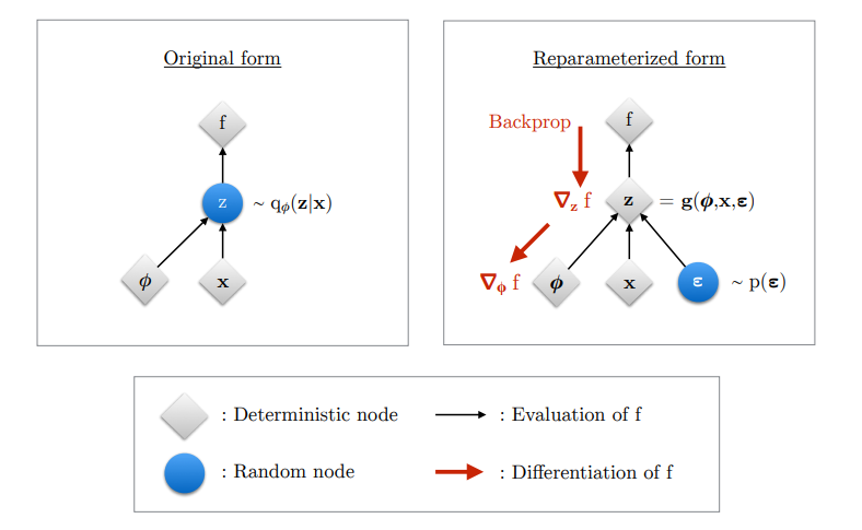
Figure 2.3 from "An Introduction to Variational Autoencoders"

Reparameterization introduces an intermediary function $g$ such that instead of $z \sim q_\phi(z|x)$, $z = g(\phi, x, \epsilon)$ where the stochasticity is delegated to random variable $\epsilon \sim p(\epsilon)$. The desired parameter for backpropagation, $\phi$, now becomes deterministic and provides a more reliable flow downstream. On a more tangible level this converts a lot of the headache witnessed in equations 5.X to something more approachable because, by reparameterizing $z$, the parameters of the density of the expectation changes, which in turn allows the gradient to be inside the expectation.

\begin{align} \nabla_\phi\mathbb{E}_{q_\phi(z|x)}[f(z)] & = \nabla_\phi\mathbb{E}_{p(\epsilon))}[f(g(\phi, x, \epsilon))] && \text{where } z = g(\phi, x, \epsilon), \epsilon \sim p(\epsilon) \\[2ex] & = \mathbb{E}_{p(\epsilon))}[\nabla_\phi f(g(\phi, x, \epsilon))] \\[2ex] & \approx \nabla_\phi f(g(\phi, x, \epsilon)) && \text{Monte Carlo estimate where } \epsilon \sim p(\epsilon) \end{align}

With reparameterization, the two representations of the variational lower bound $\mathcal{L}$ shown in "Starting with: Bayes Rule" are called the Stochastic Gradient Variational Bayes Estimator (SGVB) and can be represented as:

$$\begin{align} \mathcal{L} & \approx \mathcal{\widetilde{L}}^A \\ & = \frac{1}{L}\sum_{l=1}^L \log{p_\theta(x, z^l)} - \log{q_\phi(z^l|x)} && \text{where } z^l = g(\phi, x, \epsilon^l) \text{ and } \epsilon^l \sim p(\epsilon) \\ & \text{and} \\[2ex] \mathcal{L} & \approx \mathcal{\widetilde{L}}^B \\ & = - D_{\mathbb{KL}}(q_\phi(z|x)\,||\,p_\theta(z)) + \frac{1}{L}\sum_{l=1}^L\log{p_\theta(x|z^l)} && \text{where } z^l = g(\phi, x, \epsilon^l) \text{ and } \epsilon^l \sim p(\epsilon) \\ & = \frac{1}{2}\sum_i\Biggl(\log{\sigma_i^2} + 1 - \sigma_i^2 - \mu_i^2\Biggr) + \frac{1}{L}\sum_{l=1}^L\log{p_\theta(x|z^l)} && \text{sub in eq 4.5} \end{align}$$